Implementing distributed grid search for deep learning using TensorFlow, scikit-learn, and joblib

Michael Heilman (@heilman13) Data Scientist, Civis Analytics (@CivisAnalytics) 2016-08-28

What is this talk about?

It's about combining open source technologies to implement a machine learning workflow.

1. custom machine learning
   • TensorFlow
2. a standard interface for machine learning
   • scikit-learn
3. simple distributed computing
   • joblib

1. Custom machine learning

• ML implementation is getting easier, almost like writing equations on a whiteboard.
• The focus here: supervised, discriminative deep learning with gradient-based optimization
  • alternatives: tree ensembles, probabilistic graphical models (PyMC3, STAN), etc.

Background: Supervised, Discriminative Machine Learning

Goal: find a function $f(y \mid X, W)$ that...

• has parameters: weights $W$
• takes input: features $X$ (e.g., word counts)
• produces output: labels $y$ (e.g., positive/negative sentiment)

Procedure for finding a good $f$

Typically, we use gradient-based optimization.

1. Define an objective function $g(X, y, W)$
   • $X$, $y$: training data (fixed)
   • Goal: find setting for $W$ that optimizes $g$.
   • Often, $g$ is a difference between $\hat{y} = f(y \mid X, W)$ and $y$.
2. Define a function to compute the derivative of $g$ with respect to $W$.
   • This often duplicates engineering effort from implementing $f$ and $g$.
   • For DL models, $g$ and its derivative can be very complicated.
3. Iterate:
   • Compute the derivative.
   • Update $W$ based on the derivative.
     • Often with complex adjustments to reduce required iterations.

Graph-based numerical computation (e.g., TensorFlow)

• step 1 (model and objective implementation) becomes pretty easy
• step 2 (differentiation) becomes one line of code
• step 3 (iterative learning) becomes one or a few lines of code

TensorFlow and the alternatives

• TensorFlow's graph-based approach to numerical computation facilitates DL implementation.
  • Developed by Google, now an open source project.
  • It's pretty popular:

There are alternative DL tools, in Python (often with C++ underneath) and other languages.

• theano (Python)
  • very similar predecessor to TF
  • academic research project
• keras (Python)
  • wraps TF and theano
  • mainly for neural nets & deep learning
• mxnet (Python)
• torch (Lua)
• just NumPy + SciPy
  • scipy.optimize is handy for many things
  • no autodiff
• caffe
  • pycaffe
• Microsoft CNTK
• others
  • there's probably a new one as you read this slide.

A brief introduction to TensorFlow

"""
This is an example of accumulating a sum of 1-D tensors,
to illustrate some major concepts in TensorFlow
(variables, operations, graphs, and sessions).
"""

import numpy as np
import tensorflow as tf

# A graph is a collection of tensors and operations on them.
g = tf.Graph()

# When you create tensors and operations, they are added to
# whatever the current default graph is.
# TF lets you use context managers rather than, e.g.,
# having to do something like g.add(variable).
# Note: there is also a global default graph (global scope).
with g.as_default():

    # Define a placeholder for input (which gets added to g).
    x = tf.placeholder(dtype=np.float32, name="x")
    
    # Make a variable, including an initializer (here just a constant value).
    # Its value will be kept across calls to `run` within a session (more below).
    sum_x = tf.Variable([0., 0., 0.], name="sum_x")
    
    # You need to make sure variables are initialize in a session.
    init_op = tf.initialize_all_variables()
    
    # Make an Operation to add the input to the sum.
    # This is also added to the graph.
    # Note: the value returned by this op this will be `sum_x`.
    add_x = sum_x.assign(sum_x + x)
    
    # Sessions are execution contexts. They capture, e.g.,
    # the values of Variable instances in the graph.
    # Analogy: think of a tf.Graph as like a UNIX script/program/executable
    # and a tf.Session as like a UNIX process. It's not a perfect analogy.
    with tf.Session() as sess:
        
        # Sessions consist of multiple runs, so perhaps the run sequence
        # is the script in the analogy above.
        sess.run(init_op)
        print("session 1, initial:",
              sess.run(sum_x))
        
        print("session 1, after call 1:",
              sess.run(add_x, feed_dict={x: [1, 2, 3]}))
        
        print("session 1, after call 2:",
              sess.run(add_x, feed_dict={x: [0, 5, 0]}))
        
        print("session 1, final:",
              sess.run(add_x, feed_dict={x: [0, -10, 0]}))

session 1, initial: [ 0.  0.  0.]
session 1, after call 1: [ 1.  2.  3.]
session 1, after call 2: [ 1.  7.  3.]
session 1, final: [ 1. -3.  3.]

# Now start another session. The previous state (variable values) is lost.
# Note how we don't have to double indent as above.
with g.as_default(), tf.Session() as sess:
    # If `init_op` isn't called again, we get an exception because
    # the variable hasn't been initialized.
    sess.run(init_op)

    print("session 2, initial sum_x:", sess.run(sum_x))
    print("session 2, after call 1:",
          sess.run(add_x, feed_dict={x: [1, 1, 1]}))

session 2, initial sum_x: [ 0.  0.  0.]
session 2, after call 1: [ 1.  1.  1.]

"""
Here's a quick illustration of automatic differentiation.
Note that TensorFlow implements learning algorithms that use this internally,
to make it easy to apply various gradient-based optimizers.
"""

g = tf.Graph()
with g.as_default(), tf.Session() as sess:
    a = tf.constant([[2.0, 5.0]])
    x = tf.Variable([[0.0, 0.0]])
    y = a * x + 10.0
    y_grad = tf.gradients([y], [x])[0]  # inputs/outputs lists
    sess.run(tf.initialize_all_variables())
    print("Derivative of y = a * x + 10.0 with respect to x:\n",
          sess.run(y_grad))

Derivative of y = a * x + 10.0 with respect to x:
 [[ 2.  5.]]

Multilayer Perceptrons (MLPs)

• a feed-forward neural network
  • e.g., no recursion, no convolutions
  • input layer, 1+ hidden layers, output layer
• can model interactions between features
  • capable of approximating any function ("universal approximation theorem")
• an old idea (Rosenblatt, 1961), but can be used with state-of-the-art methods
  • e.g., ReLUs, dropout, Adam learning algorithm

$$y = f(g(x^T W_1)^T W_2$$$$f = \textrm{softmax}$$$$g = \textrm{sigmoid}$$

Notes:

• Here, we have a softmax output function $f$, for multiclass classification.
• ReLU hidden units could also be used, but they might be less interpretable than sigmoid hidden units.

2. A standard interface for machine learning

We want to follow a standard to facilitate:

• use in existing scikit-learn-based workflows
• easy comparisons to other methods in scikit-learn

The scikit-learn Estimator API

• scikit-learn is a ML library developed by many people
• The consistent API makes trying different ML algorithms easy.
• It allows users to implement their own estimators.
  • helper functions for input validation, preprocessing, testing, etc.
  • key feature: sklearn.utils.estimator_checks.check_estimator to check API conformity of a custom estimator (free tests!)
• It facilitates 2 big ML challenges:
  • pipelines of transformations
    • e.g., extract features, transform/standardize values, fit model
  • gridsearch over hyperparameters (more on this later)

Overview for custom scikit-learn predictive models

• For models, we need to implement a fit(X, y) and predict(X)
  • optionally, also predict_proba(X), etc.
• __init__ should just attach arguments
  • fit does a lot of what __init__ normally does
  • fit usually sets instance attributes (e.g., model.coef_)
• everything should be serializable with pickle
  • joblib, used by grid search, expects things to be serializable
• mixins for different model types
  • RegressorMixin, ClassifierMixin

The Civis MLP Implementation

• follows scikit-learn's API
• GPU support through TensorFlow
• sparse and dense matrix support
• generic base class + regressor and classifier subclasses
  • classifier supports binary, multiclass, and multilabel binary classification
• called MuFFNN (Multilayer Feed-Forward Neural Network)
  • https://github.com/civisanalytics/muffnn

A few alternative MLP implementations

• sklearn.neural_network.MLPClassifier (and MLPRegressor)
  • CPU-only, no GPU support
  • may be difficult to customize (e.g., new learning algorithms)
• tensorflow.learn
  • included with TensorFlow in a contrib section
  • doesn't quite follow scikit-learn interface (last I checked)
    • e.g., __init__ does more than attach arguments
    • possibly difficult to use with grid search and pipelines
  • extra support for out-of-core, minibatch learning (DataFeeder classes)
• keras.wrappers.scikit_learn.KerasClassifier
  • If you implement a model using keras, this can make it follow scikit-learn's API.
  • possibly slightly less flexible than TensorFlow.

The MLP base class

Note: I've removed some code and most documentation here for simplicity.

class MLPBaseEstimator(BaseEstimator, metaclass=ABCMeta):

    def _preprocess_targets(self, y):
        # Subclasses can override this to store information about the targets.
        return y

    def fit(self, X, y, monitor=None):
        ...        
        y = self._preprocess_targets(y)

        self.graph_ = Graph()
        with self.graph_.as_default():

            # Define the model (We'll get to this in a minute).
            self._init_model()

            # Initialize weights.
            self._session = tf.Session()
            self._session.run(tf.initialize_all_variables())
            ...

        # Minibatch training.
        for epoch in range(self.n_epochs):
            random_state.shuffle(indices)
            for start_idx in range(0, n_examples, batch_size):

                # Make the dictionary assigning a minibatch of training
                # examples (pair of arrays) to TensorFlow placeholders.
                batch_ind = indices[start_idx:start_idx + batch_size]
                feed_dict = self._make_feed_dict(X[batch_ind],
                                                 y[batch_ind])

                # Compute objective function and gradients and  update weights.
                obj_val, _ = self._session.run(
                    [self._obj_func, self._train_step],
                    feed_dict=feed_dict)

            ...

        return self

Abstract methods to be implemented by the regressor and classifier classes

...
    @abstractmethod
    def _init_model_output(self, t):
        pass

    @abstractmethod
    def _init_model_objective_fn(self, t):
        pass

    @abstractmethod
    def predict(self, X):
        pass

The core MLP modeling code

...
    def _init_model(self):
        # A placeholder variable to control dropout for training vs. prediction.
        self._dropout = \
            tf.placeholder(dtype=np.float32, shape=(), name="dropout")

        # Input layers.
        if self.is_sparse_:
           ...
        else:
            self._input_values = \
                tf.placeholder(np.float32, [None, self.input_layer_sz_],
                               "input_values")
            t = self._input_values

        # Hidden layers (self.hidden_units is a list of ints for HL sizes)
        for i, layer_sz in enumerate(self.hidden_units):
            if self.is_sparse_ ...:
                ...
            else:
                t = tf.nn.dropout(t, keep_prob=self._dropout)
                t = _affine(t, layer_sz, scope='layer_%d' % i)
            t = t if self.activation is None else self.activation(t)

        # The output layer and objective function depend on the model.
        t = self._init_model_output(t)
        self._init_model_objective_fn(t)

        # Set the training algorithm, which is currently not configurable.
        self._train_step = tf.train.AdamOptimizer().minimize(self._obj_func)
        ...

# You can't pickle some TensorFlow objects, at least as of version 0.10.0rc0.

import pickle

try:
    g = tf.Graph()
    pickle.dumps(g)
except TypeError:
    print("You can't pickle a tf.Graph")

try:
    with tf.Session() as sess:
        pickle.dumps(sess)
except TypeError:
    print("You can't pickle a tf.Session.")

You can't pickle a tf.Graph
You can't pickle a tf.Session.

Methods to support pickling

• TensorFlow has a Saver class that writes models and parameters to disk.
• One can override __getstate__, the method pickle uses to get an instance's data.
• A not-so-elegent workaround to support TF pickling:
  • write the model to disk
  • read it in as bytes
  • pickle
• unpickling is the reverse

...
   # Used when saving:
   def __getstate__(self):
        # Write out the model.
        ...
        if getattr(self, '_fitted', False):
            tempfile = NamedTemporaryFile(delete=False)
            tempfile.close()
            try:
                # Serialize the model and read it so it can be pickled.
                self._saver.save(self._session, tempfile.name)
                with open(tempfile.name, 'rb') as f:
                    saved_model = f.read()
            finally:
                os.unlink(tempfile.name)
        ...

        # Note: don't include the graph since it can be recreated.
        state = dict(
            activation=self.activation,
            batch_size=self.batch_size,
            ...
        )

        # Add fitted attributes if the model has been fit.
        if getattr(self, '_fitted', False):
            state['_fitted'] = True
            state['input_layer_sz_'] = self.input_layer_sz_
            state['is_sparse_'] = self.is_sparse_
            state['_saved_model'] = saved_model
        ...

        # Return what can and should be pickled.
        return state

    # Used when loading:
    def __setstate__(self, state):

        # Set hyperparameters, which pickled in the usual way.
        for k, v in state.items():
            if k in ['saved_model']:
                continue
            self.__dict__[k] = v

        # Reinitialize a Graph and Session, and restore the saved values.
        ...
        if state['_saved_model'] is not None:
            tempfile = NamedTemporaryFile(delete=False)
            tempfile.close()
            try:
                # Write out the serialized model that can be restored by TF.
                with open(tempfile.name, 'wb') as f:
                    f.write(state['_saved_model'])
                self.graph_ = Graph()
                with self.graph_.as_default():
                    self._init_model()
                    self._session = tf.Session()
                    self._saver.restore(self._session, tempfile.name)
            finally:
                os.unlink(tempfile.name)

Classifier subclass

class MLPClassifier(MLPBaseEstimator, ClassifierMixin):
    def __init__(self, hidden_units=(256,), batch_size=64, n_epochs=5,
                 dropout=None, activation=nn.relu, init_scale=0.1,
                 random_state=None):
        self.hidden_units = hidden_units
        self.batch_size = batch_size
        ...

    def _init_model_output(self, t):
        # Determine the output layer size.
        if self.multilabel_:
            ...
        elif self.n_classes_ > 2:
            ...
        else:
            # Binary classification
            output_size = 1

        # Add the final affine transformation.
        if self.is_sparse_ ...:
            ...
        else:
            t = tf.nn.dropout(t, keep_prob=self._dropout)
            t = _affine(t, output_size, scope='output_layer')

        # Add the output layer activation function.
        if self.multilabel_:
            ...
        elif self.n_classes_ > 2:
            ...
        else:
            # Binary classification
            self.input_targets_ = tf.placeholder(tf.int64, [None], "targets")
            t = tf.reshape(t, [-1])  # Convert to 1d tensor.
            self.output_layer_ = tf.nn.sigmoid(t)
        return t

    def _init_model_objective_fn(self, t):
        if self.multilabel_:
            ...
        elif self.n_classes_ > 2:
            ...
        else:
            # Binary classification
            cross_entropy = tf.nn.sigmoid_cross_entropy_with_logits(
                t, tf.cast(self.input_targets_, np.float32))
        self._obj_func = tf.reduce_mean(cross_entropy)

    def _preprocess_targets(self, y):
        # Store a mapping between class label (e.g., strings) and indices.
        ...

    def predict_proba(self, X):
        ...

    def predict(self, X):
        ...

    ...

3. Simple distributed computing

• motivation: ML methods have lots of hyperparameters.

  • deep learning: numbers and sizes of hidden layers, etc.
  • probabilistic graphical models: parameters for priors
  • tree ensembles: depth, learning rate, samples per split, etc.

• grid search

  • try a lots of settings, pick the one leading to the best performance on held-out development data
  • often combined with $k$-fold cross-validation (e.g., scikit-learn's GridSearchCV)
  • crude but embarassingly parallel

• Alternative hyperparameter search methods exist.

  • randomized search, HyperOpt, BayesOpt, etc.
  • also parallelizable to some extent

"""
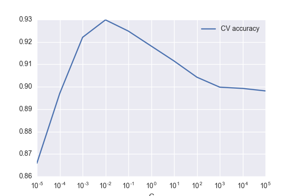
A realllllly simple illustration of how hyperparameter tuning matters.

Tuning the regularization for logistic regression on the "digits"
dataset in scikit-learn leads to a 14% error reduction in k-fold CV.
"""

import pandas as pd
from sklearn.datasets import load_digits
from sklearn.linear_model import LogisticRegression
from sklearn.grid_search import GridSearchCV
import matplotlib
import numpy as np
import matplotlib.pyplot as plt
import seaborn

digits = load_digits()
est = LogisticRegression(random_state=1234)
gs = GridSearchCV(est, param_grid={"C": [10.0 ** x for x in range(-5, 6)]})
gs.fit(digits.data, digits.target)
df = pd.DataFrame({'CV accuracy': [x.mean_validation_score
                                   for x in gs.grid_scores_],
                   'C': [x.parameters['C'] for x in gs.grid_scores_]})
df.plot(x='C', y='CV accuracy', logx=True, figsize=(6, 4))
plt.savefig('hyperparameter_search.png')

default_score = gs.grid_scores_[5].mean_validation_score
print("error reduction (k-fold CV): {0:.0f}%"
      .format(100 * (gs.best_score_ - default_score) / (1 - default_score)))

error reduction (k-fold CV): 14%

joblib

• a Python package for running embarassingly parallel tasks
  • contributors: @GaelVaroquaux, @ogrisel, et al.
• originally focused on single machine parallelization
  • backends for multiprocessing, multithreading

A simple joblib example

1. Select a backend (or use the default multiprocessing backend).
2. Instantiate a Parallel callable.
3. Call it on a bunch of delayed function calls and their arguments.

from joblib.parallel import delayed, parallel_backend, Parallel

def foo(x):
    return 10 * x ** 2

with parallel_backend("multiprocessing"):
    parallel = Parallel()
    numbers = range(10)
    print("map a function f(x)=10*x**2 over a list of numbers:\n",
          parallel(delayed(foo)(x) for x in numbers))

map a function f(x)=10*x**2 over a list of numbers:
 [0, 10, 40, 90, 160, 250, 360, 490, 640, 810]

joblib in scikit-learn

• scikit-learn uses joblib to parallelize hyperparameter evaluation in GridSearchCV
• If you tell joblib to use a custom backend, scikit-learn will use that for grid search.

joblib custom backends

• version 0.10.0 supports custom parallel backends
  • example: dask distributed backend

implementing a custom backend

• a class representing a pending result
  • similar to a concurrent.Future
  • get method to block and retrieve the result
  • result attribute to cache the result
• a joblib._parallel_backends.ParallelBackendBase subclass
  • effective_n_jobs method that determines how many jobs can run in parallel
    • e.g., can be used to cap the number of cores used across a cluster
  • apply_async method
    • queues up computation of a function call
    • returns a result instance (see above)

Civis's computation infrastructure

• Civis has an autoscaling EC2- and Docker-based system for running jobs.
  • alternatives: kubernetes, mesos
• Jobs are independent (currently, at least).
• We have a Python client with a concurrent.futures.Executor interface.
  • This allows us to submit docker run commands to remote workers.
  • We'll use a joblib backend to facilitate getting functions and data to the workers.

Outline of our backend implementation

class _CivisBackend(ParallelBackendBase):
    def __init__(self, ...):
        ...

        # Initialize an executor for making and running Docker containers.
        self.executor = ContainerPoolExecutor(**executor_kwargs)
        ...

    def effective_n_jobs(self, n_jobs):
        # e.g., set a hard limit on the number of jobs.
        ...

    def apply_async(self, func, callback=None):
        ...

        with TemporaryDirectory() as tempdir:
            # Serialize func to a temporary file and upload it to Civis.
            ...

            # Make a command for the remote Docker container that will run
            # a script that will download the serialized function `func`,
            # run it, and store the result.
            cmd = (...
                   "python {runner_script} {func_file_id}"
                   ...)
            ...

            # Submit the command to be executed in a remote Docker container.
            future = self.executor.submit(cmd)
            ...

            # Wait for the job to finish.
            result = _CivisFutureResult(future, callback)

        return result


class _CivisFutureResult:
    def __init__(self, future, callback):
        ...

    def get(self):
        if self.result is None:
            ...

            # Wait for the script to complete.
            self._future.result()

            ...

            # Download and deserialize the result.
            with TemporaryDirectory() as tempdir:
                temppath = os.path.join(tempdir, "civis_joblib_backend_result")

                # Download the serialized result.
                ...
                self.result = joblib.load(temppath)
            ...

        return self.result

Does it work?

1. Evaluate the MLP vs. logistic regression in terms of model accuracy.
2. Evaluate grid searching on my laptop versus distributed in the #cloud in terms of wall time.

A basic evaluation for text classification

• Pang & Lee (ACL 2004) Movie Reviews dataset
  • 2,000 movie reviews with positive/negative (0/1) sentiment polarity labels
• features
  • character $n$-grams from sklearn's CountVectorizer
• Evaluation setup:
  • randomly split 75% for training, 25% for testing
  • hyperparameter grid search on the training set
  • evaluate with the ROC AUC score of testing set predictions

import nltk
from nltk.corpus import movie_reviews
import numpy as np
from sklearn.linear_model import LogisticRegression
from sklearn.pipeline import Pipeline
from sklearn.cross_validation import ShuffleSplit
from sklearn.feature_extraction.text import CountVectorizer
from sklearn.grid_search import GridSearchCV
from sklearn.metrics import get_scorer
from muffnn import MLPClassifier

# Load the movie reviews data
# (polarity dataset v2.0 here: http://www.cs.cornell.edu/people/pabo/movie-review-data/).
nltk.download('movie_reviews')
X = np.array([movie_reviews.raw(i) for i in movie_reviews.fileids()])
y = np.array([1 if x.split('/')[0] == 'pos' else 0
              for x in movie_reviews.fileids()])
splits = ShuffleSplit(X.shape[0],  n_iter=1, test_size=0.25, random_state=1234)
train_ind, test_ind = [x for x in splits][0]

[nltk_data] Downloading package movie_reviews to
[nltk_data]     /Users/civisemployee/nltk_data...
[nltk_data]   Package movie_reviews is already up-to-date!

# character n-grams and a Multilayer Perceptron classifier
ct_vect = CountVectorizer(analyzer='char', ngram_range=(2, 5),
                          max_features=50000)
mlp = MLPClassifier(n_epochs=10, random_state=42)
pipeline = Pipeline(steps=[('char_ngram', ct_vect),
                           ('mlp', mlp)])
param_grid = {
    'mlp__hidden_units': [(512,), (256,), (256, 128, 64)],
    'mlp__dropout': [None, 0.5]
}
gs_mlp = GridSearchCV(pipeline, param_grid=param_grid,
                      n_jobs=4, scoring='roc_auc')

# baseline: character n-grams and a logistic regression classifier
ct_vect = CountVectorizer(analyzer='char', ngram_range=(2, 5),
                          max_features=50000)
lr = LogisticRegression(random_state=42)
pipeline = Pipeline(steps=[('char_ngram', ct_vect),
                           ('lr', lr)])
param_grid = {
   'lr__C': [0.001, 0.01, 0.1, 1.0, 10.0, 100.0]
}
gs_lr = GridSearchCV(pipeline, param_grid=param_grid,
                     n_jobs=4, scoring='roc_auc')

%time gs_lr.fit(X[train_ind], y[train_ind])
%time gs_mlp.fit(X[train_ind], y[train_ind])

CPU times: user 27.5 s, sys: 876 ms, total: 28.3 s
Wall time: 4min
CPU times: user 9min 1s, sys: 4min 54s, total: 13min 55s
Wall time: 51min 32s

roc_auc_scorer = get_scorer('roc_auc')
print("Logistic Regression ROC AUC: {:.4f}".format(
      roc_auc_scorer(gs_lr, X[test_ind], y[test_ind])))
print("MLP ROC AUC: {:.4f}".format(
      roc_auc_scorer(gs_mlp, X[test_ind], y[test_ind])))

Logistic Regression ROC AUC: 0.9119
MLP ROC AUC: 0.9271

With distributed grid search

factory = make_backend_factory(
    required_resources={"cpu": 2048, "memory": 4096}, ...)
register_parallel_backend('civis', factory)

with parallel_backend('civis'):
    gs_mlp.fit(X[train_ind], y[train_ind])

Wall time:

• laptop: 51min 32s
• distributed: 16min 23s

Notes: both include refitting on all the data locally after grid search.

Parting thoughts (speculation)

• With deep learning, speeding up hyperparameter search is important.
• Distributed grid search > distributed model fitting
  • (probably, currently, for many applications)
• When combining open-source tools, whole > np.sum(parts)

Thanks

• Matt Becker, Bill Lattner, Derrick Higgins (for code review)
• Walt Askew (for code contributions)